What,Why, and How...

Quantization is a critical concept in the fields of artificial intelligence (AI) and machine learning (ML), especially as these technologies continue to evolve. This article delves into what quantization is, its necessity, and its impact on AI and ML models.

What is Quantization?

Quantization refers to the process of minimizing the number of bits required to represent a number. In practice, this often involves converting floating-point representations in higher precision formats to lower precision formats. This can include converting an array or weight matrix or model that is in FP32 to FP16, or INT4, or INT8 representations. This process is an essential component of model compression strategies, along with other techniques such as pruning, knowledge distillation, and low-rank factorization.

Why Do We Need Quantization?

The need for quantization arises from several challenges associated with AI and ML models:

1. Size of Models: Contemporary AI models are often large, requiring substantial storage and computational resources for training and inference.

2. Memory and Energy Efficiency: Floating-point numbers, commonly used in AI models, require more memory and are less efficient in terms of energy consumption compared to integer representations.

Benefits of Quantization

1. Improved Inference Speed and Reduced Memory Consumption: Quantization primarily works by converting floating-point numbers to integers. This transformation not only reduces the overall size of the model, making it more compact and storage-efficient, but also significantly enhances the speed of inference. The integer-based operations are simpler and faster compared to their floating-point counterparts, leading to quicker computations. This is especially beneficial in real-time applications where rapid data processing is crucial. Additionally, with the reduced memory footprint, the models become more manageable, particularly in constrained environments like mobile devices or edge computing scenarios.

2. Enhanced Computational Speed: Quantization accelerates computation, particularly during inference, due to the simpler mathematical operations required for integers compared to floating points.

3. Energy Efficiency: With a more compact model size and faster computation, quantization contributes to lower energy consumption.

4. Edge Computing: The reduced size and increased efficiency make it feasible to run sophisticated models on edge devices and smartphones.

By addressing the challenges posed by the size and complexity of AI models, quantization serves as a key enabler for the more efficient and widespread use of AI and ML technologies.

Quick example

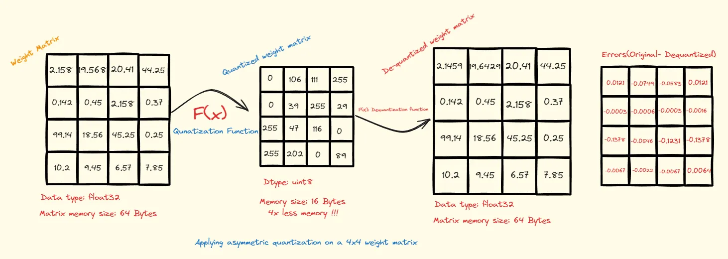
Consider the example illustrated below, where we have a 4x4 weight matrix. These weights are initially stored as 32-bit floating-point numbers, which is a standard data type for such operations, consuming a total of 64 bytes. Our goal is to reduce this footprint while retaining as much of the original information as possible.

Click here to see code:

# Your Python code goes here
import torch

w = [
    [2.158,19.568,20.41,44.25],
    [0.142,0.45,2.158,0.37],
    [99.14,18.56,45.25,0.25],
    [10.2,9.45,6.57,7.85]
    ]
w = torch.tensor(w)

def asymmetric_quantization(weight_matrix, bits, target_dtype= torch.uint8):
    alphas = (weight_matrix.max(dim=-1)[0]).unsqueeze(1)
    betas = (weight_matrix.min(dim=-1)[0]).unsqueeze(1)
    scale = (alphas - betas) / (2**bits-1)
    zero = -1*torch.round(betas / scale)
    lower_bound, upper_bound = 0, 2**bits-1

    weight_matrix = torch.round(weight_matrix / scale + zero)
    weight_matrix[weight_matrix < lower_bound] = lower_bound
    weight_matrix[weight_matrix > upper_bound] = upper_bound

    return weight_matrix.to(target_dtype), scale, zero

def asym_dequant(weignt_matrix,scale,zero):

    return (weignt_matrix-zero)*scale

w_quant,scale,zero = asymmetric_quantization(w, 8)
w_dequant = asym_dequant(w_quant, scale, zero)

print('Original Matrix is: \n',w,'\n\n','Quantized Matrix is: \n',w_quant,'\n\n'\
      'De-quantized is \n',w_dequant,'\n')

original_size_in_bytes= w.numel()*w.element_size()
Qunatized_size_in_bytes= w_quant.numel()*w_quant.element_size()

print(f'Size before quantization: {original_size_in_bytes} \nSize after quantization: {Qunatized_size_in_bytes}')

To achieve compression, we employ a quantization function that maps the original floating-point values to a specified range. In this case, we utilize an asymmetric quantization range of 0-255, corresponding to the uint8 data type. This choice is strategic; an asymmetric range ensures that we can capture the full scope of values without resorting to a larger data type like int32, which would negate the size benefits.

As a result, the quantized matrix holds values ranging from 0 to 255, and the total memory consumed is now only 16 bytes—a reduction to a quarter of the original size. Furthermore, by applying a dequantization function, we can translate these integers back into floating-point numbers. On the far right, we see the error matrix, comparing the original and dequantized values, with most discrepancies being imperceptibly close to zero.

This example offers a succinct introduction to the process of quantization. We’ve explored the basics, and now it’s time to delve deeper into the specific types within the broader category of Range-Based Linear Quantization—namely, asymmetric and symmetric quantization.

Range-Based Linear Quantization

Asymmetric Quantization
Symmetric Quantization

Asymmetric Quantization

In asymmetric quantization, we transform floating-point numbers or vectors from their original range, typically denoted as , into a new, narrower range defined by . Here, represents the bit depth; is the minimum, and is the maximum value within the array or vector. For example, in our prior discussion, we chose to be 8 because we worked with the uint8 data type, which spans 8 bits and covers a value range from 0 to 255.

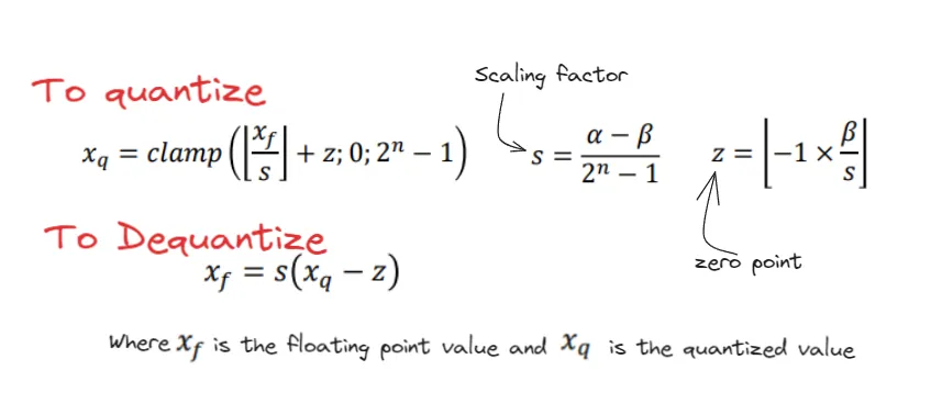
Let’s examine the formula that facilitates this conversion from floating-point numbers to their quantized counterparts within the specified asymmetric range:

The term is known as the zero point. Essentially, it represents a mapping of the zero point from a source vector to a quantized vector. This means it maps the zero point in a floating number to an equivalent new number in the quantized series. Consider the following example:

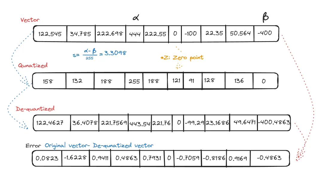
From the example we discussed, we see that the number 0 is mapped to 121, which we call the zero point. When we de-quantize, two key parameters come into play: scale and zero point. The scale depends on two values, and , which represent the maximum and minimum values of our vector. However, there’s a catch. If any of these points are outliers, they can cause quantization errors. You might have noticed this in the error vector - it’s not all zeros as we would expect.

To tackle this, one strategy is to use percentiles, like the 99th or 10th, for determining the max and min values. Ultimately, our goal is to minimize the error between the reconstructed array and the original one. Another important aspect of asymmetric quantization is understanding the range. The minimum value from the original data is mapped to zero, and the maximum value is mapped to , where (n) is the bits used for quantization.

Now, let’s explore Symmetric Quantization.

Symmetric Quantization

In symmetric quantization, we map the entire floating-point vector to a range that is equidistant on both sides of the zero point. This range extends equally in both negative and positive directions. To determine the mapping range, we first find the maximum absolute value in the vector, which we call . This gives us a mapping range of . Our quantized range then becomes , where (n) is the number of bits used for quantization.

let’s delve into formula,

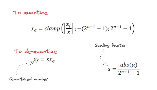
As compared to asymmetic quantization, we don’t have any zero point here,zero is mapped to zero, let’s consider an example:

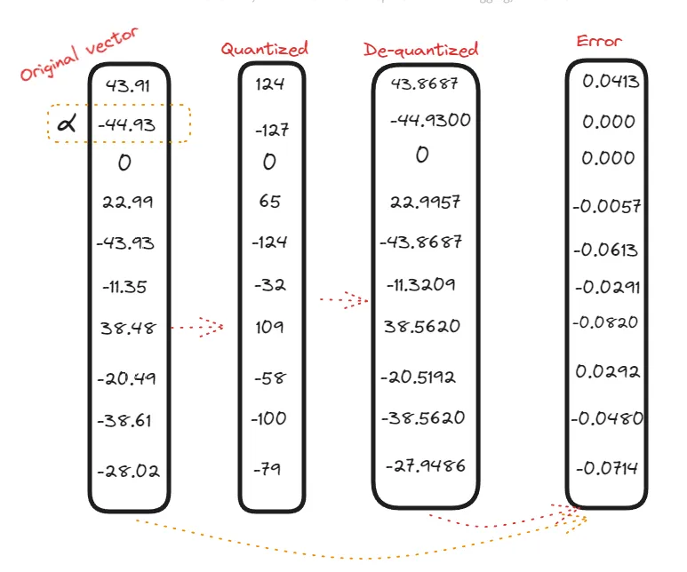
In symmetric quantization, it is evident that values within the negative domain remain in the negative domain even after quantization. Additionally, the zero point remains consistent in both vectors or mappings.

Click here to see code:

torch.set_printoptions(sci_mode=False)
def symmetric_quantization(weight_matrix, bits, target_dtype= torch.int8):
    alphas = (weight_matrix.abs().max(dim=-1)[0]).unsqueeze(1)
    scale = (alphas) / ((2**(bits-1))-1)

    lower_bound, upper_bound = -(2**(bits-1)-1), (2**(bits-1))-1

    weight_matrix = torch.round(weight_matrix / scale)
    weight_matrix[weight_matrix < lower_bound] = lower_bound
    weight_matrix[weight_matrix > upper_bound] = upper_bound

    return weight_matrix.to(target_dtype),scale

def symmetric_dequantization(weight_matrix,scale):
    return weight_matrix*scale

w = [[43.91, -44.93,0,22.99,-43.93,-11.35,38.48,-20.49,-38.61,-28.02],
    [56.45,0,125,22,154,0.15,-125,256,36,-365]]

w = torch.tensor(w)


w_quant,scale = symmetric_quantization(w, 8)
w_dequant = symmetric_dequantization(w_quant, scale)



print('Original Matrix is: \n',w,'\n\n','Quantized Matrix is: \n',w_quant,'\n\n'\
      'De-quantized is \n',w_dequant,'\n')

original_size_in_bytes= w.numel()*w.element_size()
Qunatized_size_in_bytes= w_quant.numel()*w_quant.element_size()

print(f'Size before quantization: {original_size_in_bytes} \nSize after quantization: {Qunatized_size_in_bytes}')

An important aspect to consider is that both of these quantization methods are susceptible to outliers. This is because the scale factor is dependent on the range, and the presence of outliers can significantly impact the errors. To mitigate this, various strategies can be employed. One approach is to determine the maximum and minimum values based on percentiles. Another strategy involves selecting the max and min values from a specified range, such as . This can be achieved through methods like grid search, which aim to minimize the mean squared error In addition to the Mean-Squared-Error (MSE) approach, where we choose parameters and to minimize the MSE between the original and quantized values, Cross-Entropy plays a crucial role in certain scenarios. This method is particularly relevant when quantizing tensors in which not all values hold equal importance. A prime example is found in the Softmax layer of Large Language Models (LLMs). In these models, maintaining the hierarchy of the most significant values post-quantization is vital due to the reliance on inference strategies like Greedy, Top-P, or Beam search. Therefore, the goal becomes to find and that minimize the Cross-Entropy between the original softmax values and the quantized softmax values, ensuring that the order of the largest values is preserved after quantization.

Beyond Linear Qunatization

Beyond these, the field of quantization is rich with diverse methods, each suited to different scenarios and requirements. For instance, DorEfa and WRPN are two other notable techniques that have emerged, offering unique approaches to reducing model size and computational overhead. While our current discussion centers on Range-Based Linear Quantization, it’s important to acknowledge these other methodologies as well. Future articles will delve into DorEfa and WRPN, providing a comprehensive understanding of the landscape of quantization in machine learning.

Next, let’s turn our attention to how these quantization techniques are actually used. We’ll take a closer look at methods like Post-Training Quantization (PTQ) and Quantization Aware Training (QAT), which are key to making machine learning models more efficient and effective. Join me as we explore these important techniques and their practical applications.